GSW2020 - Photos and material

You can see here some photos of the GEOframe Winter School 2020. The material and the final refine OMS/GEOframe GWS2020 project can be found on

• Zenodo: https://zenodo.org/record/3627007#.Xir75CN7nb0. 

It contains all the needed input and output files for executing the School's project. It will not work if you do not do all the right operation. Therefore, please browse the school material in order starting from the first post.

Previous Winter School Page                      All pages                           First Page

GWS2020 - The Bonus II: Richards equation treated better better than in Hydrus 1D

The second bonus of the GEOframe Winter School on GEOframe is about the Richards' equation. Here we present the ongoing work by Niccolò Tubini (AboutHydrology) in his doctorate. In particular he is presenting how his code is working and why we believe it is a good code.

The presentation by Niccolò is divided into 2 parts: I and II.  The illustrated Jupyter Notebook as wells as the codes can be dowloaded from Github. There you can find also the Jupyter Notebooks and also browse the other software, including the Richards1D version coupled with the energy budget.

Previous Winter School page

All Winter School pages

Next Winter School page 

GWS2020 - The Bonus I: A little on Travel Times

In the last days of the GEOframe WinterSchool 2020, most of the time was dedicated to simulating with the software but we also give a little clue on  topics that we could not expand more. This is the case of travel times modelling (and/or residence time).  Here Marialaura Bancheri (GS, Abouthydrology) talks a little about the theory and the applications she did mainly in her thesis.

You can watch the video of her talk here.  So far we did just the application that can be seen In Marialaura's thesis which are mostly demonstrative that real. Soon, however, in the project WATZON, we will use them massively.

Previous Winter School page

All Winter School pages

Next Winter School page 

GWS2020 - Rainfall Runoff

Here we are introducing some modules for rainfall runoff modelling present in GEOframe.  We also maintain some material of the 2019 GEOframe Winter School that can be though interesting.

• The GEOframe type of models (YouTube2020)
• Representing the Hydrological Dynamical Systems (YouTube2020)
• The Embedded Reservoir Model (YouTube2020)
• The ERM sim file (Part I, II, III)
• The Net3 Graph
• LUCA calibration of the ERM
• Examples of Application
• The Posina Catchment (Abera et al., 2017a)(YouTube2019)
• The Blue Nile (Abera et al. 2017b) (YouTube2019)
• The Basilicata Civil Protection (YouTube2019)

• Net3 (YouTube2020)
• LUCA (YouTube2020)

Cavone River Exercise

• Part I (YouTube2020), Part II (YouTube2020), Part III (YouTube2020)

Goodness of fit notebooks

• Here

General references to Rainfall-Runoff

Beven, K. (2012), Ranfall Runoff, the primer, Wiley-Blackwell

Rigon, R., Bancheri, M., Formetta, G., & de Lavenne, A. (2015). The geomorphological unit hydrograph from a historical-critical perspective. Earth Surface Processes and Landforms, http://doi.org/10.1002/esp.3855

References besides the one already used

For seeing how to represent lumped hydrological models (you can give a look to this paper here)

Abera, W.W. (2016), Modelling water budget at a basin scale using JGrass-NewAge system. PhD thesis, University of Trento

Bancheri, Marialaura (2017) A flexible approach to the estimation of water budgets and its connection to the travel time theory. PhD thesis, University of Trento.


Bancheri, M., Serafin, F., & Rigon, R. (2019). The Representation of Hydrological Dynamical Systems Using Extended Petri Nets (EPN). Water Resources Research, 8(01), 159–27. http://doi.org/10.1029/2019WR025099

Bancheri, M., Rigon, R., & Manfreda, S. (2020). The GEOframe-NewAge Modelling System Applied in a Data Scarce Environment. Water, 12(1), 86–24. http://doi.org/10.3390/w12010086

Formetta, Giuseppe (2013) Hydrological modelling with components: the OMS3 NewAge-JGrass system. PhD thesis, University of Trento.

Formetta, G., Antonello, A., Franceschi, S., David, O., & Rigon, R. (2014). Hydrological modelling with components: A GIS-based open source framework, 55(C), 190–200. http://doi.org/10.1016/j.envsoft.2014.01.019

Patta, C, Costruzione di un modello idrologico di stima della disponibilità idrica in area pedemontana, Tesi di laurea (in Italian), Politecnico di Torino, 2018

For open questions about rainfall-runoff see also the Meledrio Posts.

Previous Winter School page

All Winter School pages

Next Winter School page 

GWS2020 - Evaporation and Transpiration

Evapotranspiration accounts for most of fifty percent of the terrestrial hydrological cycle. We illustrate here some ways to estimate it with the tools offered by the GEOframe system. 

Radiation

We do not cover radiation in this school. We will just use it. For people interested, however, they can give a look to the material of 2019 School here.


The 2020 material

• Momentum and water vapor transport in atmosphere (YouTube2020)
• Evaporation as energy flow (YouTube2020)
• Derivation of the simplified energy budget (a là Penman-Monteith after Schymanski and Or) (YouTube2020)
• Simplified relatives of PMSO (YouTube2020)
• Leaf Temperature feedbacks
• Transpiration (YouTube2020)
• Further discussions on resistances and the physiology of plants in this video. 
• Evaporation from soil (YouTube2020)
• From leaves to canopies (YouTube2019 Video, YouTube2020)

The 2019 material

• Momentum and water vapor transport in atmosphere (YouTube2019)
• Penman-Monteith according to Shymanski and Or (PMSO- YouTube2019)
• PMSO with surfaces temperatures feedbacks (YouTube 2019)
• Evaporation from soil and Traspiration mechanisms (YouTube2019)
• From leaves to canopies (YouTube2019 Video)
• Documentation of GEOframe-NewAge component 2019
• Jupyter notebook with exercises
• Live YouTube video on the sim files and Jupyter notebooks

Out of schedule (for Chhay)

• Budyko curves derivation

Exercises

• You can follow this Jupyter notebook

References

Primarily for historic papers browse to the list by Dennis Baldocchi

• Haghighi, E., Shahraeeni, E., Lehmann, P., & Or, D. (2013). Evaporation rates across a convective air boundary layer are dominated by diffusion. Water Resources Research, 49(3), 1602–1610. http://doi.org/10.1002/wrcr.20166
• Lehmann, P., Assouline, S., & Or, D. (2008). Characteristic lengths affecting evaporative drying of porous media. Physical Review E, 77(5), 354–16. http://doi.org/10.1103/PhysRevE.77.056309
• Lehmann, P., & Or, D. (2013). Effect of wetness patchiness on evaporation dynamics from drying porous surfaces. Water Resources Research. http://doi.org/10.1002/2013WR013737
• Or, D., Lehmann, P., & Shahraeeni, E. (2013). Advances in soil evaporation Physics - A review. Vadose Zone Journal.
• Schymanski, S. J., & Or, D. (2017). Leaf-scale experiments reveal an important omission in the Penman–Monteith equation. Hydrology and Earth System Sciences, 21(2), 685–706. http://doi.org/10.5194/hess-21-685-2017
• Schymanski, S. J., Or, D., & Zwieniecki, M. (2013). Stomatal Control and Leaf Thermal and Hydraulic Capacitances under Rapid Environmental Fluctuations. PLoS ONE, 8(1), e54231–16. http://doi.org/10.1371/journal.pone.0054231
• Shokri, N., & Or, D. (2011). What determines drying rates at the onset of diffusion controlled stage-2 evaporation from porous media? Water Resources Research, 47(9), 584–8. http://doi.org/10.1029/2010WR010284
• Stroock, A. D., Pagay, V. V., Zwieniecki, M. A., & Michele Holbrook, N. (2014). The Physicochemical Hydrodynamics of Vascular Plants. Annual Rev. Fluid Mech., 46(1), 615–642. http://doi.org/10.1146/annurev-fluid-010313-141411

See also the discussions here:

• The vapour budget
• Soil-Plants fluxes
• Stomatal resistance and Evapotranspiration

And the mini-series: 

• The man who planted trees.

Previous Winter School page

All Winter School pages

Next Winter School page 

The Jupyter notebooks and OMS project repository for the WSG2020

During the classes we use several Jupyter notebooks. You can find them at the appropriate OSF page:

Jupyter Notebooks

So if you search a notebook and you do not know where to find them: they are here.

The OMS project used is instead here:

Overall OMS3 project (available on Zenodo). It contains all the software used in the school.

GWS2020 - Delineating catchments

The second day of the Winter School on GEOframe is dedicated to the watershed delineation and hillslope extraction. First the relevant concepts are given. Then GEOframe (Horton Machine) tools are used to get the desired results.

We recovered something from the first day.

• Hydrogeomorphology: the basic theory (YouTube video 2019,YouTube2020)
• OMS-Horton Machine tools description:
• Aspect
• Curvature
• Cutout
• Pitfiller
• Slope/Gradients
• TC or Topographic classes
• Hydrogeomorphology: the derived quantities (YouTube video 2019,YouTube2020)
• OMS-Horton Machine tools description:
• ExtractNetwork
• Flow Directions/Draindir
• MarkOutlet
• Water Outlet
• Hydrogeomorphology: extracting the hillslope (YouTube Video 2019,YouTube2020)
• Network ordering
• OMS-Horton Machine tools description:
• Network Attributes Builder
• A little on some geomorphic laws (YouTube video 2019, YouTube2020)
• Example: the Cavone case (Basilicata)
• Videos of the afternoon lab 
• Part I
• - (not very visible but understandable)
• Part II - (not very visible but understandable)
• Part III - (not very visible but understandable)
• Part IV - (not very visible but understandable)
• Part V 
• Part VI
• Part VII
• Part VIII 
• Again on using QGIS for dividing Cavone Catchment into subbasins (part I, part II, part II)
• The Horton Machine in gvSIG (not treated at the school but an interesting complement)
• Using QGIS for obtaining the centroids of subbasins  (YouTube video 2019)

References

• Various information from the AboutHydrology Blog
• Rigon, R., I. Rodriguez-Iturbe, A. Rinaldo, A. Maritan, A. Giacometti and D. Tarboton, On Hack’s law, Water Resources Research, 32(11), 3367, 1996
• R.Rigon, E. Ghesla, C. Tiso and A. Cozzini, The Horton Machine, pg. viii, 136, ISBN 10:88-8443-147-6, University of Trento, 2006
• W. Abera, A. Antonello, S. Franceschi, G. Formetta, R Rigon , "The uDig Spatial Toolbox for hydro-geomorphic analysis" in Geomorphological Techniques, v. 4, n. 1 (2014), p. 1-19

Previous Winter School page

All Winter School pages

Next Winter School page 

GWS2020 - Getting Started with OMS and Jupyterlab

Day first of the Winter School on GEOframe was conceived to give people the taste of what OMS is and how to use it with Python lab. For the Installations, please refer to the Installation page. 

Not much information about Jupyterlab though. It will be given interactively using notebooks and explaining their contents.

• The philosophy behind OMS/GEOframe (YouTube video 2019, YouTube2020)
• The GEOframe deployment (YouTube2020)
• A brief introduction to the Object Modelling System (YouTube video 2019,YouTube2020, Also on VIMEO2020)
• OMS User Manual - Introduction (pdf, epub) 
• The OMS working environment (YouTube video 2020)
• OMS User Manual - The working Environment (pdf, epub)
• The structure of a .sim file (YouTube video 2019, YouTube2020)
• The existing manual excerpt (outdated but still useful) (pdf, epub)
• The OMS console (YouTube2020)
• Examples 2020.
• Examples 2019 (All the material in the .zip files. Notebooks in /docs folder)
• ex_00 (zip files)
• Examples-basic (zip files). Please find Jupyter notebook shown in video below in the doc directory of the zipped files.
• Example 001 (YouTube video 2019)
• Controlling Iteration (Ex 05) YouTube video 2019.
• Going on with examples: Again on You Tube Video Iteration, Bulk connect, Feedbacks
• Exercises 1&2
• Watertank  Example (zip files). Documentation in the doc folder.
• Water Tank example - Part I YouTube video 2019
• Exercises 3&4
• Creating a notebook from the scratch (Live YouTube video 2019 by Niccolò Tubini)

Previous Winter School page

All Winter School pages

Next Winter School page 

Installing Java and OMS

The Winter School on the GEOframe system is approaching.  In this post you will find all the preparatory material of the school indexed.

Installations

You are not assumed to know Python or Java to participate to the School. However programs GOFRAME programs runs on Java 8. Input/Output of models will be treated by using some scripting in Python. We will communicate the appropriate notions during the classes but the interested can finfd plenty of courses on the web (for instance this comes from SciPy 2018. Other from SciPy here.)

• Java. GEOframe and OMS are written in Java and they require to have installed Java on your computer. Here you can find instructions to install Java on your computer.  OMS need Java 8 JDK.  Please note that you need the Java Development Toolkit (JDK) installed not the Java Runtime Environment (JRE).  You can watch several videos for Windows here but Windows user can follow our previous blogpost.  For Macs, look at here. Googling you can get more videos and information. 
• OMS v 3 Console. It is possible to use Docker to execute the programs but, after the experience of the last year with Docker installations on Windows, we preferred to use directly the Console. The OMS system installation traditional information can be found here: https://alm.engr.colostate.edu/cb/wiki/16961 and https://alm.engr.colostate.edu/cb/wiki/17107.  During the School we will use the Console 3.6.28. To install the Console, you have to download and unzip it, put it in a directory (folder) of your choice.  A new directory called oms-3.6.28-console will be created, inside of which you'll see:

• To start the Console from Windows, just click on the .bat file
• To start the Console from Mac OSX or Linux, open a Terminal and execute:
• % ./console.sh &
• The "&" just free the command line back and gives it back to you. 

• During the School we will use Jupyter and Python 3 for data management and visualisation. It would be great if you could arrive with Jupyter installed.
• The post at this link contains all the information needed. For installation of the software, we suggest Anaconda. For any problem contact us through the mailing list https://groups.google.com/forum/#!forum/geoframe-winter-schools. 
• To understand what a Jupyter notebook is about, please see its manual. However, we will use Jupyterlab.  (You can see a YouTube video about here).  One can think that Jupyter was heavily based on the look-and-feel of Mathematica notebooks: but Jupyterlab is a step ahead to something different. Installing Anaconda, you also have already installed Jupyter notebook. You can open Jupyter lab by the Anaconda Console, or issuing the command  Jupyter lab at a terminal (called DOS prompt in Windows).

• The manual of Jupyterlab is here.
• BTW, it will be useful to have also a GIS of your choice installed. We suggest QGIS.

Set the Java Home in the Console

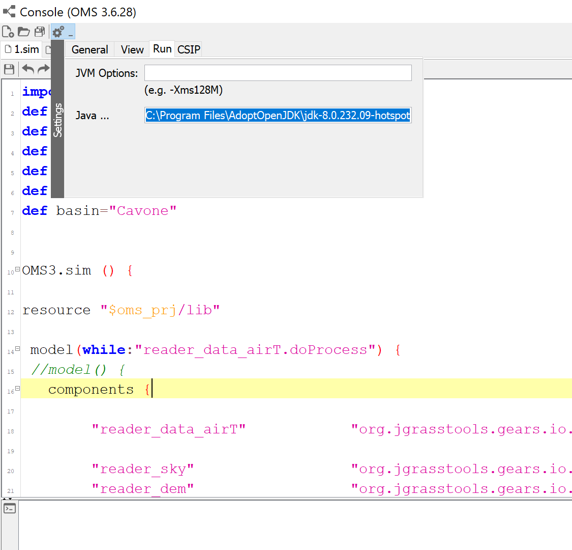
• Just open the pull-down menù below from the first Console Window  (you must just click on the plus sign on the fourth icon on top left) and then insert in the Java Home the full path of your Java Home (if you do not know where it is, look at here: MS Windows, Mac/Linux)

New: The OMS project and software used during the school is here on Zenodo. Download it for using it later according to the what you will find on the next pages.

Previous Winter School page

All Winter School pages

Next Winter School page

How to install the Object Modelling System Console on Windows 10

1) Download openJDK 8 LTS from

https://adoptopenjdk.net/

2) Install it

3) Open a command prompt and run the command:

java -version

It should return:

openjdk version "1.8.0_232"
OpenJDK Runtime Environment (AdoptOpenJDK)(build 1.8.0_232-b09)
OpenJDK 64-Bit Server VM (AdoptOpenJDK)(build 25.232-b09, mixed mode)

4) Download the Object Modeling System console version 3.6.28 from

https://alm.engr.colostate.edu/cb/wiki/16961

5) Unzip the Object Modeling System console and run the console.bat file

6) In the console setting, select the panel Run and set the Java path (see screenshot) to the previously installed JDK which usually is:

C:\Program Files\AdoptOpenJDK\jdk-8.0.232.09-hotspot

(please check the correct JDK version first)

GEOframe Winter School 2020 - It is time to apply !

The second edition on the Winter School on GEOframe will be held between January 8 and 17, 2020 in Trento, Italy.  The course is devoted to Ph.D. Students, Post-docs, Young researchers (and Professionals!) interested in estimating all the components of the hydrological cycle (rainfall, evapotranspiration, snow-melting, and river discharge).  The system they will learn allows to work out very small catchments and continental basins as well (e.g. Abera et al., 2017a,b) up to build operational solutions as the one used in in Basilicata.

The aim of the course is to enable participants to run their own simulations and eventually on their own catchments and estimate the hydrological budget components.
With respect to the 2019 Winter School, there will be more practice and more detailed work on evapotranspiration and rainfall-runoff. It will be much more focused on exercises and on getting the water budget performed under various hypotheses on models' structure.

Website for the enrollment go here.

For the hole definitive material of the School go here. 

The provisional topics will be:

Teachers will be:

Prof. Riccardo Rigon, Ph.D.

Prof. Giuseppe Formetta, Ph.D.

Marialaura Bancheri, Ph.D.
Niccolò Tubini, Ph.D. student

The topics (links added after the School):

• Day 1 -   Installation of the Infrastructure and Jupyter - Getting started with OMS and Jupyter lab (Rigon, Formetta, Tubini)
• Day 2-   Hydrologic Response Units delineation and treatment of spatial features (Rigon, Formetta, Tubini).
• Day 3/4- Interpolation of hydrometeorological datasets and elements of parameters calibration with LUCA and particle swarm tools ((Rigon, Formetta, Tubini)
• Day 5 - Estimation of evaporation and transpiration  (Bancheri, Rigon, Formetta, Tubini)
• Day 6/7 - Rainfall-Runoff (Bancheri, Rigon, Formetta, Tubini)
• Day 8 - A little on Travel Times - Richards Equation 1D (Bancheri,  Formetta, Tubini)

To have an idea of the topics, the interested researchers should give look at the material (slides, video etc. of the 2019 Winter School).  The material of the first three days remains very similar (but refined) to the old one. Therefore, for students is possible also to participate only to the second week (at the same cost, but saving some lodging) but, in that case, is mandatory to follow the on-line courses and tutorials  relative of 8-9-10 January topics and having done the exercises before December 15. We will offer prompt online support to them up to that date and no support whatsoever on the same topics later or  between 13-17 of January for clear reasons of course efficiency and organisation.  The refined material of the first three days will be available on the Winter School website  from November 15, 2019.

With respect to the 2019 School, there will be more practice and more detailed material on Evapotranspiration and Rainfall-Runoff. For every 40 minutes of talk there will be 70 minutes of supervised exercise for a total of 8 hour a day of activities. 

Cost of the School is 350 Euros for who will subscribe before November 15, 400 Euros for others. A discount of 20 Euros is granted to fellows of the Italian Hydrological Society (subscriptions for students are available at the IHS-SII site for 10 Euros to students and 20 to seniors). Who attended the last year school can participate free of charge, upon subscription. Inclusive of the costs will be coffee breaks and lunch at the Cafeteria of Department of Civil, and one social dinner for all the schoolmates Environmental and Mechanical Engineering. 

Website for the enrollment go here.

For any further information, please fill free to contact me at riccardo.rigon <at> unitn.it